Project aim
Recover continuous deformation phase from noisy, wrapped interferograms, including the low-coherence regimes where classical unwrappers struggle, without ever producing a result that contradicts the data.
- 99.1%Exact cycle count, easy test scenes
- 96.6%Exact cycle count, moderate test scenes
- 92.0%Full-scene skill, easy (oracle = 100)
- ≤ 3 ptsTrain–validation gap at every difficulty
Phase unwrapping is where most InSAR errors are born. pyunwrap learns the integer cycle count rather than the phase itself, so every answer stays consistent with the radar measurement.
What is new
- 1
Predict the integer, not the phase
Unwrapping is posed as per-pixel classification of the cycle count k. The output is consistent with the input by construction, so the network cannot invent phase that was never measured.
- 2
Physics-informed training objective
An ambiguity term, with optional re-wrap, smoothness and residue terms. The run shown here is ablation A, ambiguity term only, which sets the baseline the physics terms must beat.
- 3
Tile, stitch and align
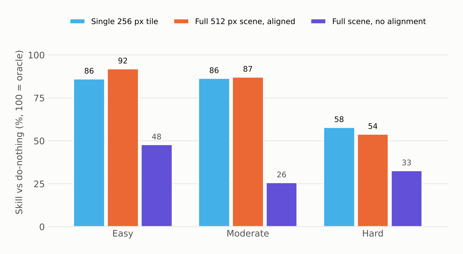
The network works on 256 px tiles; full scenes are reassembled with overlap and per-tile cycle alignment. Alignment lifts full-scene skill on easy scenes from 47.8% to 92.0%.
- 4
Difficulty curriculum
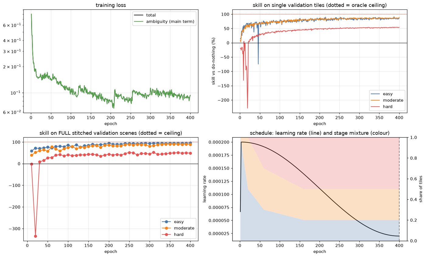
Training starts on easy scenes and shifts to a 20 / 30 / 50 easy / moderate / hard mix, while the hard-scene coherence level ramps from 0.6 down to 0.3 between epochs 30 and 300.
- 5
Regime-aware routing
SNAPHU and the learned model are combined region by region, based on which one benchmarks stronger, rather than claiming one method always wins.
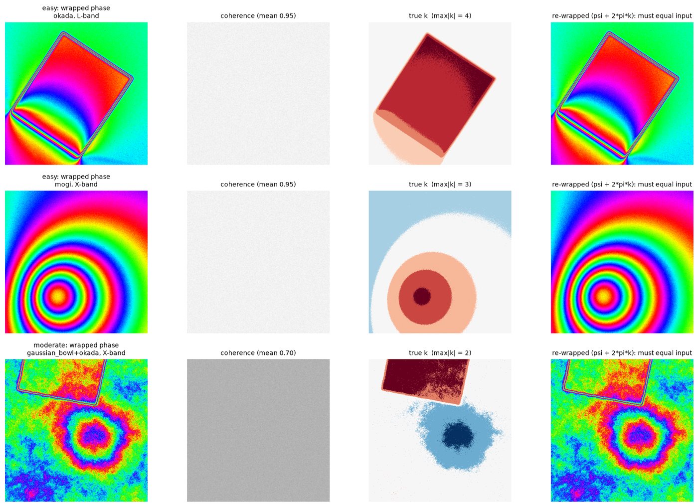
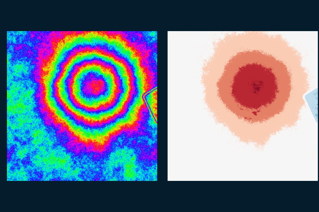 Real run output: wrapped input and predicted cycle map
Overview
Phase unwrapping turns a wrapped interferogram, whose values only span −π to π, into continuous phase; any error here propagates into every deformation map built on it. pyunwrap's AmbiguityNet does not regress phase directly. It predicts the integer number of 2π cycles, k, at each pixel. Because the unwrapped phase is the wrapped input plus 2πk, re-wrapping the output always reproduces the observed interferogram exactly. At scene level, pyunwrap routes each region to SNAPHU or to the learned model, whichever its benchmarks show is stronger.
The challenge
Low coherence from vegetation, long temporal baselines or steep deformation creates phase residues, and classical path-following and network-flow unwrappers can propagate a single cycle error across a whole scene. Learned unwrappers that regress continuous phase have the opposite problem: they can drift away from the measurement itself. The goal was to learn from data while keeping the physical constraint exact, and to work on scenes larger than the tiles the network sees in training.
Data & inputs
Approach
-
01
Simulate realistic interferograms
Synthetic 512 × 512 scenes with three deformation sources (Gaussian subsidence bowls, Mogi volcanic point sources and Okada fault dislocations) at L-, C- and X-band, with a 4-look speckle noise model and spatially varying coherence.
-
02
Encode the physics in the target
The label is the true integer cycle map k; a re-wrap check on every training example confirms that ψ + 2πk reproduces the input.
-
03
Train with a curriculum
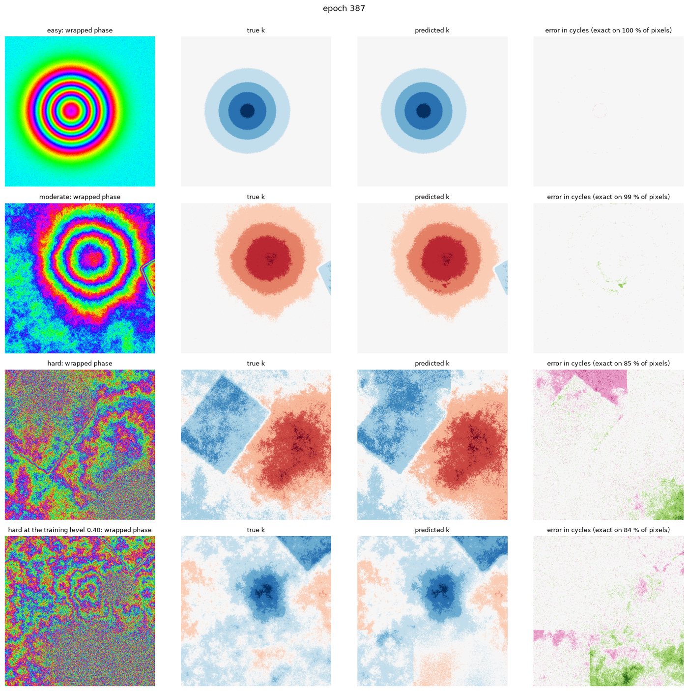
400 epochs of 1,200 tiles each, batch 8, peak learning rate 2 × 10⁻⁴ with warm-up and cosine decay, mixing difficulty levels over time. The best checkpoint came at epoch 387.
-
04
Predict, stitch and align
Tiles overlap by 64 px in training and 128 px at inference; predictions are stitched into full scenes with cycle alignment between tiles.
-
05
Measure against an oracle
Skill is scored against a do-nothing baseline (0) and the oracle (100), together with the share of pixels whose cycle count is exactly right, across a sweep of coherence levels.
-
06
Route by regime
At scene level, regions go to SNAPHU or to AmbiguityNet depending on which performs better under the local conditions.
Model & training setup
| Model | AmbiguityNet: per-pixel classification of integer cycle count k |
|---|---|
| Training data | Synthetic interferograms: 80 easy, 80 moderate, 400 hard scenes (512 × 512) |
| Deformation sources | Gaussian bowl, Mogi point source, Okada fault |
| Bands & noise | L-, C- and X-band; speckle, 4 looks |
| Tiling | 256 px tiles; 64 px overlap in training, 128 px at inference |
| Schedule | 400 epochs × 1,200 tiles, batch 8, peak LR 2e-4, cosine to 10% floor |
| Curriculum | Easy → 50/50 → 30/40/30 → 20/30/50 mix; hard coherence 0.6 → 0.3 |
| Loss (this run) | Ambiguity term only (ablation A) |
| Selected checkpoint | Epoch 387 of 400 |
| Hardware | Single CUDA GPU |
Benchmark
| Difficulty | Tile skill | Full-scene skill | Full scene, no alignment | Exact cycles |
|---|---|---|---|---|
| Easy | 86.1% | 92.0% | 47.8% | 99.1% |
| Moderate | 86.4% | 87.2% | 25.7% | 96.6% |
| Hard | 57.9% | 53.9% | 32.7% | 80.0% |
Figures from the run
Results
On held-out test scenes, 99.1% of pixels receive exactly the right cycle count on easy scenes, 96.6% on moderate and 80.0% on hard. Full stitched scenes reach 92.0%, 87.2% and 53.9% of oracle skill, and training and validation skill stay within 3 points of each other at every level, so the model generalises to unseen scenes rather than memorising them. By deformation type, Mogi sources are easiest (97.5% full-scene skill on easy scenes) and Okada faults, with their sharp discontinuities, are hardest.
Validation
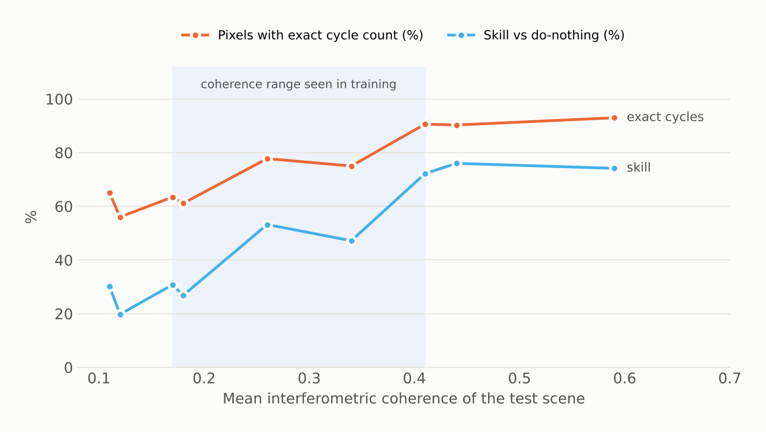
Separate validation and test scene sets (12 per difficulty level), a coherence sweep from 0.80 down to 0.20, breakdowns by deformation source, and a train-versus-validation check. The CV records that, on the project's own benchmarks, SNAPHU wins on most scenes and the learned model wins under low-coherence decorrelation, which is why pyunwrap routes rather than replaces.
Limitations, stated plainly
- These results are on synthetic interferograms. Real-scene performance has to be established scene type by scene type.
- Skill falls steeply below a mean coherence of about 0.35, to roughly 20–30% of oracle skill at the lowest levels tested.
- Fault discontinuities (Okada sources) remain the hardest case: 53.1% full-scene skill on hard scenes with faults versus 62.0% without.
- This run is the ambiguity-only ablation. The contribution of the re-wrap, smoothness and residue terms is measured in separate ablation runs.