pyunwrap: Learned InSAR Phase Unwrapping
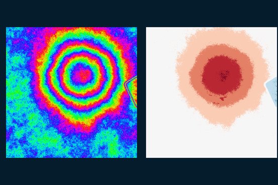
A network that predicts the integer 2π cycle count at every pixel, so it can never contradict the measured phase. 99.1% of pixels exact on easy test scenes, 96.6% on moderate.
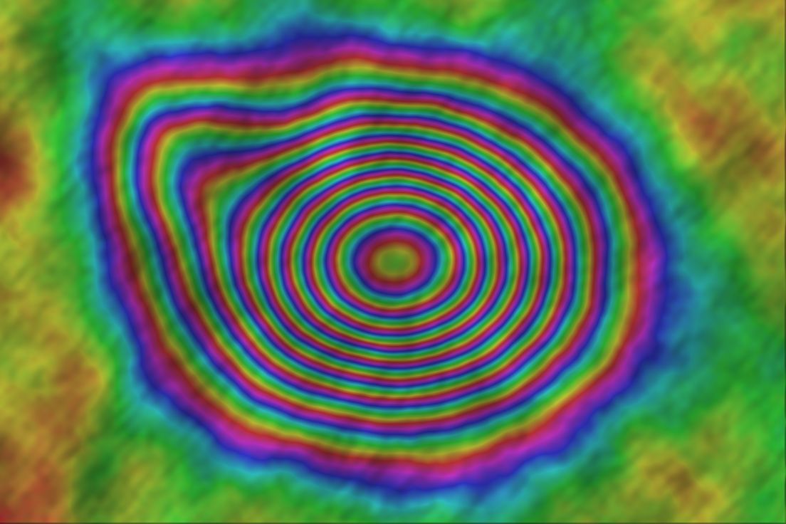
Radar satellites see through cloud and darkness, and interferometric SAR (InSAR) turns the phase difference between acquisitions into ground displacement. I build and run complete Sentinel-1 chains, from SLC search to SBAS velocity maps, for land subsidence, infrastructure stability and earthquake and volcanic deformation.
Tracking urban subsidence from groundwater extraction, construction or reclamation.
Screening roads, dams, embankments and mine sites for slow, hidden movement.
Measuring deformation after earthquakes and eruptions with a reproducible chain.
Where persistent cloud cover makes optical monitoring unreliable.
Expected rate, spatial extent and the decision it informs. These set the stack length, acquisition geometry and the choice between SBAS and persistent-scatterer methods.
Preflight checks on AOI coverage, network connectivity and perpendicular and temporal baselines catch a doomed stack before compute is spent.
Orbit-based coregistration with per-burst Enhanced Spectral Diversity, flat-earth and topographic phase removal, ERA5 tropospheric and IONEX ionospheric correction.
SNAPHU by default; pyunwrap's learned unwrapper where low coherence defeats it. Each region is routed to the method that benchmarks stronger, rather than claiming one method always wins.
SBAS inversion to velocities and time series; graph-neural-network persistent-scatterer selection (ps-gnn) for irregular urban targets.
Compare with published references, GNSS or levelling where available, and report network fragmentation and coherence gaps alongside the map.
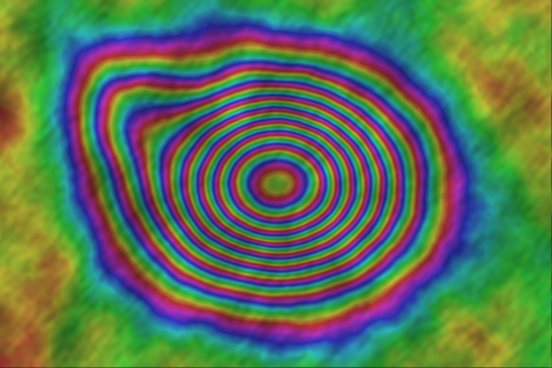
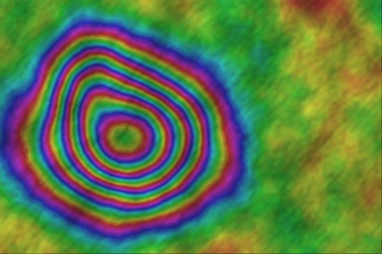
Mexico City subsidence, the 2021 Piton de la Fournaise eruption and the 2016 Amatrice earthquake were processed with the same pygeofetch InSAR chain.
A network that predicts the integer 2π cycle count at every pixel, so it can never contradict the measured phase. 99.1% of pixels exact on easy test scenes, 96.6% on moderate.
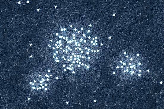
Persistent-scatterer selection as node classification on a spatial graph. F1 0.82 vs 0.69 for StaMPS-style selection on hard test scenes, and 0.97 recall on borderline scatterers.
67 SLC scenes; 2,211 candidate pairs reduced to 78 valid interferograms; −35.5 to −2.9 cm/yr, consistent with the peer-reviewed −39.1 cm/yr peak.
Sentinel-1 from the ASF Vertex API through an SBAS chain, with a Tiny U-Net on an 8-channel stack exported to ONNX for edge deployment.
Connectivity, coherence and fragmentation are part of every deliverable, so you know how far to trust each pixel.
Classical and learned unwrapping are combined region by region, based on benchmarks rather than preference.
The full Sentinel-1 workflow lives in pygeofetch, CI-tested and archived with a DOI, so results can be reproduced.